Feature Matching + Homography to find a known object
In this sample, you will use features2d and calib3d to detect an object in a scene.
You will learn how to:
- Use the function cv.findHomography to find the transform between matched keypoints.
- Use the function cv.perspectiveTransform to map the points.
Sources:
Contents
In a previous demo, we used a queryImage, found some feature points in it, we took another trainImage, found the features in that image too and we found the best matches among them. In short, we found locations of some parts of an object in another cluttered image. This information is sufficient to find the object exactly on the trainImage.
For that, we can use a function from calib3d module, cv.findHomography. If we pass the set of points from both the images, it will find the perpective transformation of that object. Then we can use cv.perspectiveTransform to find the object. It needs atleast four correct points to find the transformation.
We have seen that there can be some possible errors while matching which may affect the result. To solve this problem, algorithm uses Ransac or LMedS (which can be specificed in the Method option). So good matches which provide correct estimation are called inliers and remaining are called outliers. cv.findHomography returns a mask which specifies the inlier and outlier points.
Options
OPTS_FEATURE = 'SURF';   % detector: ORB, BRISK, AKAZE, KAZE, SIFT, SURF
OPTS_FLANN = true;       % matcher: FLANN or Brute Force
OPTS_KNN_MATCH = false;  % matcher method: match or knnMatch (k=2)
Input images
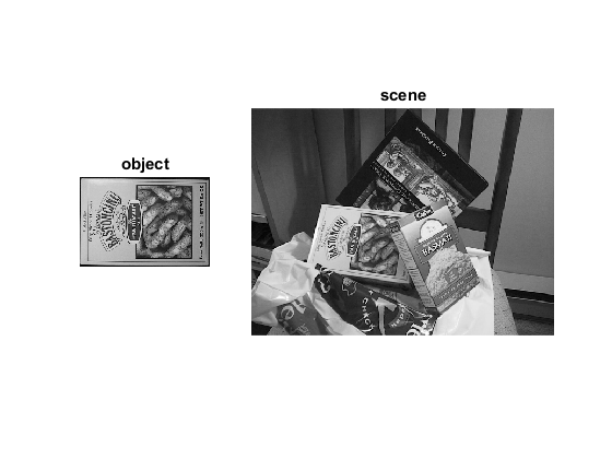
imgObj = cv.imread(fullfile(mexopencv.root(),'test','box.png'), 'Grayscale',true);
imgScene = cv.imread(fullfile(mexopencv.root(),'test','box_in_scene.png'), 'Grayscale',true);
subplot(1,3,1), imshow(imgObj), title('object')
subplot(1,3,[2 3]), imshow(imgScene), title('scene')

Step 1: Detect the keypoints and extract descriptors using SURF
switch upper(OPTS_FEATURE)
    case 'SURF'
        detector = cv.SURF('HessianThreshold',400);
    case 'SIFT'
        detector = cv.SIFT();
    case 'ORB'
        detector = cv.ORB();
    case 'BRISK'
        detector = cv.BRISK();
    case 'AKAZE'
        detector = cv.AKAZE();
    case 'KAZE'
        detector = cv.KAZE();
    otherwise
        error('unrecognized feature: %s', OPTS_FEATURE)
end
display(detector)
detector =
  SURF with properties:

                  id: 2
    HessianThreshold: 400
            NOctaves: 4
       NOctaveLayers: 3
            Extended: 0
             Upright: 0
[keyObj,featObj] = detector.detectAndCompute(imgObj);
[keyScene,featScene] = detector.detectAndCompute(imgScene);
fprintf('object: %d keypoints\n', numel(keyObj));
fprintf('scene: %d keypoints\n', numel(keyScene));
whos featObj featScene
object: 786 keypoints
scene: 1040 keypoints
  Name              Size             Bytes  Class     Attributes

  featObj         786x64            201216  single
  featScene      1040x64            266240  single
Step 2: Matching descriptor vectors using FLANN matcher
if OPTS_FLANN
    if ~isempty(strfind(detector.defaultNorm(), 'Hamming'))
        opts = {'LSH', 'TableNumber',6, 'KeySize',12, 'MultiProbeLevel',1};
    else
        opts = {'KDTree', 'Trees',5};
    end
    matcher = cv.DescriptorMatcher('FlannBasedMatcher', 'Index',opts);
else
    matcher = cv.DescriptorMatcher('BFMatcher', ...
        'NormType',detector.defaultNorm());
end
display(matcher)
matcher =
  DescriptorMatcher with properties:

      id: 33
    Type: 'FlannBasedMatcher'
if OPTS_KNN_MATCH
    matches = matcher.knnMatch(featObj, featScene, 2);
else
    matches = matcher.match(featObj, featScene);
end
fprintf('%d matches\n', numel(matches));
786 matches
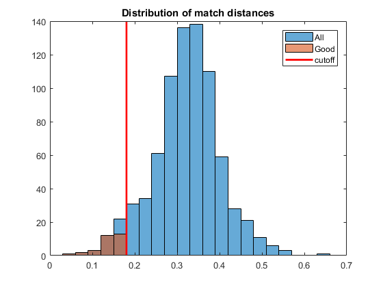
Filter matches and keep only "good" ones
if OPTS_KNN_MATCH
    % ratio test
    dists = cellfun(@(m) m(1).distance, matches);
    idx = cellfun(@(m) (numel(m) == 2) && ...
        (m(1).distance < 0.75 * m(2).distance), matches);
    matches = cellfun(@(m) m(1), matches(idx));
else
    % distance less than k*min_dist
    dists = [matches.distance];
    cutoff = 3 * min(dists);
    matches = matches(dists <= cutoff);
    fprintf('Min dist = %f\nMax dist = %f\nCutoff = %f\n', ...
        min(dists), max(dists), cutoff);
end
fprintf('%d good matches\n', numel(matches));
Min dist = 0.055168
Max dist = 0.644580
Cutoff = 0.165503
31 good matches
show original and filtered distances
if ~mexopencv.isOctave()
    %HACK: HISTOGRAM not implemented in Octave
    figure
    hh = histogram(dists); hold on
    histogram([matches.distance], hh.BinEdges)
    if OPTS_KNN_MATCH
        legend({'All', 'Good'})
    else
        line([cutoff cutoff] + hh.BinWidth/2, ylim(), 'LineWidth',2, 'Color','r')
        legend({'All', 'Good', 'cutoff'})
    end
    hold off
    title('Distribution of match distances')
end

Get the keypoints from the good matches (Note: indices in C are zero-based while MATLAB are one-based)
ptsObj = cat(1, keyObj([matches.queryIdx]+1).pt);
ptsScene = cat(1, keyScene([matches.trainIdx]+1).pt);
whos ptsObj ptsScene
  Name           Size            Bytes  Class     Attributes

  ptsObj        31x2               496  double
  ptsScene      31x2               496  double
Step 3: Compute homography
assert(numel(matches) >= 4, 'not enough matches for homography estimation');
[H,inliers] = cv.findHomography(ptsObj, ptsScene, 'Method','Ransac');
assert(~isempty(H), 'homography estimation failed');
inliers = logical(inliers);
display(H)
fprintf('Num outliers reported by RANSAC = %d\n', nnz(~inliers));
H =
    0.4283   -0.1864  121.5736
    0.0022    0.3643  162.5073
   -0.0002   -0.0005    1.0000
Num outliers reported by RANSAC = 2
Step 4: Localize the object
% get the corners from the first image (the object to be "detected")
[h,w,~] = size(imgObj);
corners = [0 0; w 0; w h; 0 h];
display(corners)

% apply the homography to the corner points of the box
p = cv.perspectiveTransform(corners, H);
display(p)
corners =
     0     0
   324     0
   324   223
     0   223
p =
  121.5736  162.5073
  282.7520  177.2785
  267.8110  299.2625
   89.2696  271.9903
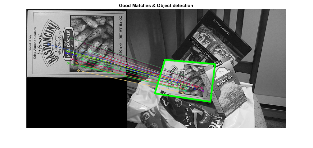
Show results
% draw the final good matches
imgMatches = cv.drawMatches(imgObj, keyObj, imgScene, keyScene, matches, ...
    'NotDrawSinglePoints',true, 'MatchesMask',inliers);

% draw lines between the transformed corners (the mapped object in the scene)
p(:,1) = p(:,1) + w;  % shift points for the montage image
imgMatches = cv.polylines(imgMatches, p, 'Closed',true, ...
    'Color',[0 255 0], 'Thickness',4, 'LineType','AA');
figure, imshow(imgMatches)
title('Good Matches & Object detection')
