Histogram Calculation

In this demo, we show how to:

Sources:

Contents

Theory

Histograms are collected counts of data organized into a set of predefined bins. When we say data we are not restricting it to be intensity values. The data collected can be whatever feature you find useful to describe your image.

Let's see an example. Imagine that a matrix contains information of an image (i.e. intensity in the range ):

What happens if we want to count this data in an organized way? Since we know that the range of information value for this case is 256 values, we can segment our range in subparts (called bins) like:

and we can keep count of the number of pixels that fall in the range of each . Applying this to the example above we get the image below (axis x represents the bins and axis y the number of pixels in each of them).

This was just a simple example of how an histogram works and why it is useful. An histogram can keep count not only of color intensities, but of whatever image features that we want to measure (i.e. gradients, directions, etc).

Let's identify some parts of the histogram:

What if you want to count two features? In this case your resulting histogram would be a 3D plot (in which x and y would be and for each feature and z would be the number of counts for each combination of . The same would apply for more features (of course it gets trickier).

For simple purposes, OpenCV implements the function cv.calcHist, which calculates the histogram of a set of arrays (usually images or image planes). It can operate with up to 32 dimensions. We will see it in the code below!

Code

This program:

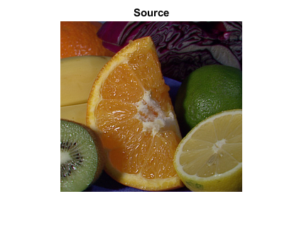
Load source 8-bit color image

img = cv.imread(fullfile(mexopencv.root(), 'test', 'fruits.jpg'), ...
    'Color',true, 'ReduceScale',2);
imshow(img), title('Source')

Calculate histogram over each channel, 8-bit values are between [0,255]

counts = zeros(256,3);
for i=1:3
    I = img(:,:,i);
    if true
        % intervals: [0,1), [1,2), ..., [254,255), [255,256)
        counts(:,i) = cv.calcHist(I, [0 256], 'HistSize',256, 'Uniform',true);
    elseif mexopencv.require('images')
        % intervals: [-0.5,0.5), [0.5,1.5), ..., [253.5,254.5), [254.5,255.5)
        counts(:,i) = imhist(I, 256);
    elseif ~mexopencv.isOctave()
        % intervals: [0,1), [1,2), ..., [254,255), [255,256]
        counts(:,i) = histcounts(double(I), 0:256);
    elseif true
        % intervals: [0,1), [1,2), ..., [254,255), [255,255]
        counts(:,i) = histc(double(I(:)), 0:255);
    elseif true
        counts(:,i) = accumarray(double(I(:))+1, 1, [256 1]);
    else
        counts(:,i) = full(sparse(double(I(:))+1, 1, 1, 256, 1));
    end
end

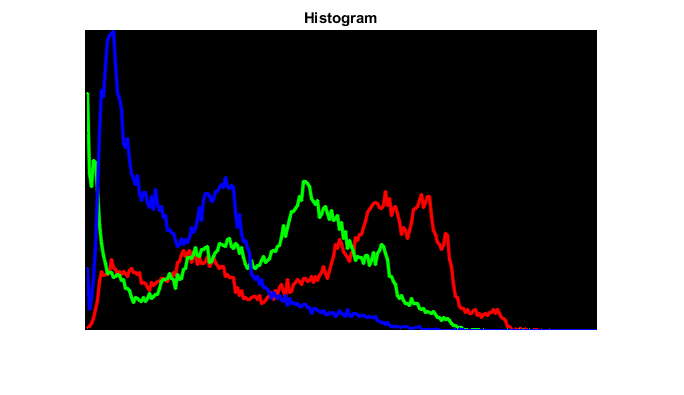
Plot 1

clrs = 255*eye(3);  % BGR
out = zeros([300 512 3],'uint8');
sz = size(out);
X = (1:256)' * round(sz(2) / 256);
Y = sz(1) - round(counts / max(counts(:)) * sz(1));
for i=1:3
    out = cv.polylines(out, [X Y(:,i)], ...
        'Closed',false, 'Color',clrs(i,:), 'Thickness',2, 'LineType','AA');
end
figure, imshow(out), title('Histogram')

Plot 2

clrs = {'r'; 'g'; 'b'};
a = [1.0, 0.7, 0.7];
if ~mexopencv.isOctave()
    %HACK: Octave doesn't have histogram function yet
    figure
    for i=1:3
        histogram('BinEdges',0:256, 'BinCounts',counts(:,i), ...
            'FaceColor',clrs{i}, 'EdgeColor','none', 'FaceAlpha',a(i))
        hold on
    end
    hold off, axis([0 256 0 Inf]), grid on
    xlabel('Intensities'), ylabel('Counts'), title('Histogram')
end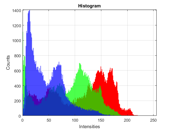

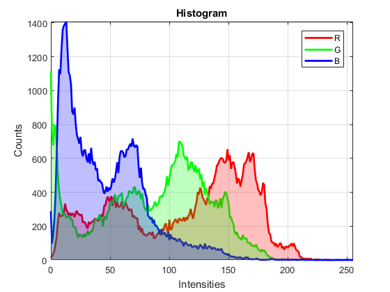
Plot 3

figure
hh = plot(0:255, counts); hold on
for i=1:3
    h = bar(0:255, counts(:,i), 'histc');
    if mexopencv.isOctave()
        %HACK: Octave returns hggroup containing the patch object
        h = get(h, 'Children');
    end
    %NOTE: FaceAlpha in Octave causes patch to become fully transparent
    set(h, 'EdgeColor','none', 'FaceColor',clrs{i}, 'FaceAlpha',0.25)
    set(hh(i), 'Color',clrs{i}, 'LineWidth',2)
end
hold off, axis([0 255 0 Inf]), grid on
xlabel('Intensities'), ylabel('Counts'), title('Histogram')
legend(hh, upper(clrs))

Plot 4

figure
for i=1:3
    subplot(3,1,i)
    h = bar(0:255, counts(:,i), 'histc');
    if mexopencv.isOctave()
        %HACK: Octave returns hggroup containing the patch object
        h = get(h, 'Children');
        %HACK: Octave creates very dense xticks 0:255
        set(gca, 'XTick',0:50:255)
    end
    if true
        % gradient color
        clr = zeros(1,256,3);
        clr(:,:,i) = (0:255)/255;
        set(h, 'EdgeColor','none', 'CData',clr)
    else
        % flat color
        set(h, 'EdgeColor','none', 'FaceColor',clrs{i})
    end
    axis([0 255 0 max(counts(:))]), grid on
    ylabel(upper(clrs{i}))
    if i==1, title('Histogram'); end
end
xlabel('Intensities')