Histogram Equalization

In this demo, we show:

Sources:

Contents

Theory

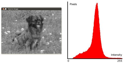
An Image Histogram is a graphical representation of the intensity distribution of an image. It quantifies the number of pixels for each intensity value considered.

Histogram Equalization is a method that improves the contrast in an image, in order to stretch out the intensity range. To make it clearer, from the image above, you can see that the pixels seem clustered around the middle of the available range of intensities. What Histogram Equalization does is to stretch out this range. Take a look at the figure below: The green circles indicate the underpopulated intensities. After applying the equalization, we get an histogram like the figure in the center. The resulting image is shown in the picture at right.

Equalization implies mapping one distribution (the given histogram) to another distribution (a wider and more uniform distribution of intensity values) so the intensity values are spreaded over the whole range. To accomplish the equalization effect, the remapping should be the cumulative distribution function (cdf) (more details, refer to Learning OpenCV). For the histogram , its cumulative distribution is:

To use this as a remapping function, we have to normalize such that the maximum value is 255 (or the maximum value for the intensity of the image). From the example above, the cumulative function is:

Finally, we use a simple remapping procedure to obtain the intensity values of the equalized image:

Code

This program:

Load source 8-bit grayscale image

if true
    im = which('pout.tif');
else
    im = which('tire.tif');
end
if isempty(im)
    im = fullfile(mexopencv.root(), 'test', 'sudoku.jpg');
end
src = cv.imread(im, 'Grayscale',true);

Apply histogram equalization

if true
    dst = cv.equalizeHist(src);
elseif mexopencv.require('images')
    dst = histeq(src);
end

Select function to plot 1D histogram

lvl = @(I) sprintf('%d unique levels', numel(unique(I(:))));
if mexopencv.require('images')
    histFunc = @imhist;
else
    histFunc = @my_imhist;
end

Display both images and their histograms

subplot(221), imshow(src), title('Source')
subplot(223), imshow(dst), title('Equalized')
subplot(222), histFunc(src), title(lvl(src))
subplot(224), histFunc(dst), title(lvl(dst))

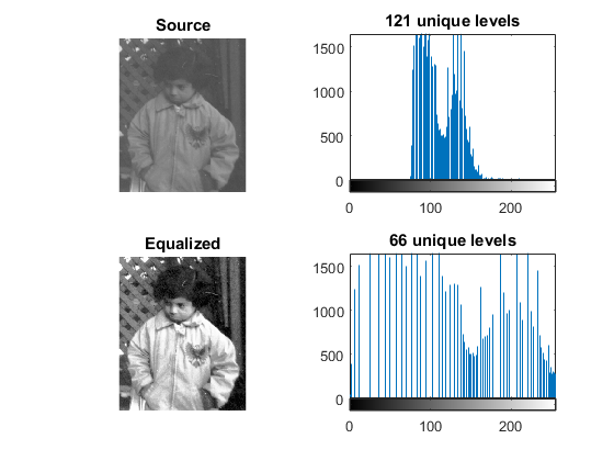
Notice that the pixels are clustered around the center of the histogram. After applying the equalization, the image has certainly more contrast. Notice how the number of pixels is more distributed through the intensity range.

Helper function

function my_imhist(I)
    % compute histogram for 8-bit grayscale image
    bins = 0:255;
    counts = histc(double(I(:)), bins);

    % plot intensities counts
    stem(bins, counts, 'Marker','none')
    axis([0 255 0 Inf])

    % plot color stripe at the bottom
    yl = round(0.05 * max(counts));
    clr = repmat(uint8(bins), [10 1 3]);
    image('XData',[0 255], 'YData',[-yl 0], 'CData',clr)
    set(gca, 'Layer','top')
    axis tight
end