Similarity measurement (PSNR and SSIM)
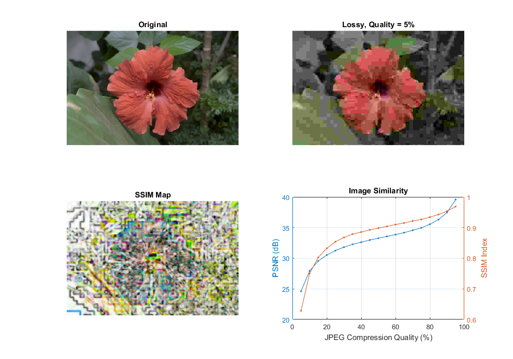
Image similarity under lossy compression.
Sources:
Contents
PSNR
We want to check just how imperceptible our compression operation went, therefore we need a system to check the similarity
or differences. The most common algorithm used for this is the PSNR (aka Peak signal-to-noise ratio). The simplest definition of this starts out from the mean squad error. Let there be two images:  and
and  ; with a two dimensional size
  and
and  , composed of
  number of channels.
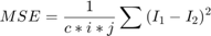
Then the PSNR is expressed as:
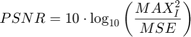
Here the  is the maximum valid value for a pixel. In case of the simple single byte image per pixel per channel this is 255. When two
images are the same the MSE will give zero, resulting in an invalid divide by zero operation in the PSNR formula. In this
case the PSNR is undefined and as we'll need to handle this case separately. The transition to a logarithmic scale is made
because the pixel values have a very wide dynamic range.
is the maximum valid value for a pixel. In case of the simple single byte image per pixel per channel this is 255. When two
images are the same the MSE will give zero, resulting in an invalid divide by zero operation in the PSNR formula. In this
case the PSNR is undefined and as we'll need to handle this case separately. The transition to a logarithmic scale is made
because the pixel values have a very wide dynamic range.
Typically result values are anywhere between 30 and 50 for compression, where higher is better. If the images significantly differ you'll get much lower ones like 15 and so. This similarity check is easy and fast to calculate, however in practice it may turn out somewhat inconsistent with human eye perception. The structural similarity algorithm aims to correct this.
SSIM
Describing the methods goes well beyond the purpose of this tutorial. For that I invite you to read the article introducing it. Nevertheless, you can get a good image of it by looking at the implementation below.
SSIM is described more in-depth in the following article:
Z. Wang, A. C. Bovik, H. R. Sheikh and E. P. Simoncelli,
"Image quality assessment: From error visibility to structural similarity"
IEEE Transactions on Image Processing, vol. 13, no. 4, pp. 600-612, Apr. 2004
This will return a similarity index averaged over all channels of the image. This value is between zero and one, where one corresponds to perfect fit. Unfortunately, the many Gaussian blurring is quite costly, so while the PSNR may work in a real-time like environment (24 frame per second) this will take significantly more than to accomplish similar performance results.
Code
Therefore, the source code presented below will perform the PSNR measurement and the SSIM. For visualization purpose we show both images with corresponding PSNR and MSSIM values.
function image_similarity_demo(fname)
    % reference image
    if nargin < 1
        fname = fullfile(mexopencv.root(), 'test', 'test1.png');
    end
    A = cv.imread(fname, 'ReduceScale',2);

    figure('Position',[100 100 1000 700]);
    subplot(221), imshow(A), title('Original')

    % compress with decreasing quality
    qual = 95:-5:5;
    vals = zeros(numel(qual), 3);
    for i=1:numel(qual)
        % lossy compression
        if true
            buf = cv.imencode('.jpg', A, 'JpegQuality',qual(i));
        else
            buf = cv.imencode('.webp', A, 'WebpQuality',qual(i));
        end
        B = cv.imdecode(buf);
        vals(i,3) = numel(buf);

        % compute similarity
        vals(i,1) = cv_psnr(A, B);
        [vals(i,2), map] = cv_ssim(A, B);

        % show result
        subplot(222), imshow(B)
        title(sprintf('Lossy, Quality = %d%%',qual(i)))
        subplot(223), imshow(map), title('SSIM Map')
        drawnow;
    end

    % plot similarities
    subplot(224)
    [ax, h1, h2] = plotyy(qual, vals(:,1), qual, vals(:,2));
    set([h1 h2], 'Marker', '.')
    title('Image Similarity')
    xlabel('JPEG Compression Quality (%)')
    ylabel(ax(1), 'PSNR (dB)')
    ylabel(ax(2), 'SSIM Index')
    grid on

    if ~mexopencv.isOctave()
        t = array2table([qual(:), vals], ...
            'VariableNames',{'Quality', 'PSNR', 'SSIM', 'Bytes'});
        disp(t)
    end
end

function val = cv_psnr(img1, img2)
    %CV_PSNR  Peak Signal-to-Noise Ratio
    %
    % See also: psnr, cv.PSNR
    %

    % validate arguments
    assert(isa(img1,'uint8') && isa(img2,'uint8'), 'images must be 8-bit');
    assert(isequal(size(img1), size(img2)), 'images must have the same size');

    % mean squared error
    se = double(cv.absdiff(img1, img2)).^2;
    mse = mean(se(:));

    % PSNR (in dB)
    val = 10.0 * log10((255*255) / mse);
    if ~isfinite(val)
        val = 0;  % division by zero MSE
    end
end

function [val, map] = cv_ssim(img1, img2)
    %CV_SSIM  Structural Similarity Index
    %
    % See also: ssim
    %

    % validate arguments
    assert(isa(img1,'uint8') && isa(img2,'uint8'), 'images must be 8-bit');
    assert(isequal(size(img1), size(img2)), 'images must have the same size');

    % constants to stabilize the division with weak denominator
    k1 = 0.01;
    k2 = 0.03;
    L = 2^8 - 1;  % 8-bit dynamic range of pixel-values
    C1 = (k1*L)^2;
    C2 = (k2*L)^2;

    % filtering options
    opts = {'KSize',[11 11], 'SigmaX',1.5, 'SigmaY',1.5};

    % work in floating-point precision
    I1 = double(img1);
    I2 = double(img2);

    % mean
    mu1 = cv.GaussianBlur(I1, opts{:});
    mu2 = cv.GaussianBlur(I2, opts{:});

    % variance
    sigma1_2 = cv.GaussianBlur(I1.^2, opts{:}) - mu1.^2;
    sigma2_2 = cv.GaussianBlur(I2.^2, opts{:}) - mu2.^2;

    % covariance
    sigma12 = cv.GaussianBlur(I1.*I2, opts{:}) - mu1.*mu2;

    % SSIM index
    map = ((2 * mu1.*mu2 + C1) .* (2 * sigma12 + C2)) ./ ...
        ((mu1.^2 + mu2.^2 + C1) .* (sigma1_2 + sigma2_2 + C2));
    val = mean(map(:));
end
    Quality     PSNR      SSIM      Bytes
    _______    ______    _______    _____
    95         39.578    0.96866    39532
    90         37.469    0.95371    27081
    85           36.3    0.94262    21329
    80         35.541     0.9339    18149
    75         34.956    0.92656    15901
    70         34.557    0.92153    14450
    65         34.176    0.91499    13234
    60         33.855    0.90994    12205
    55          33.56    0.90393    11374
    50         33.261    0.89813    10737
    45          32.97     0.8926    10121
    40         32.603    0.88531     9377
    35         32.264    0.87868     8727
    30         31.802    0.86771     7944
    25         31.243    0.85372     7127
    20         30.514    0.83233     6231
    15         29.542    0.80236     5294
    10         27.923    0.74988     4191
     5          24.61     0.6283     3088