K-Means Clustering
An example on K-means clustering.
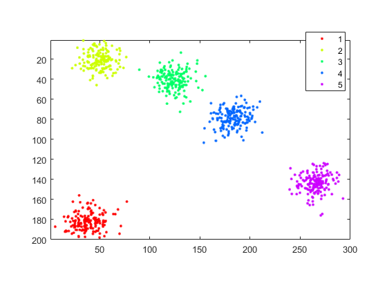
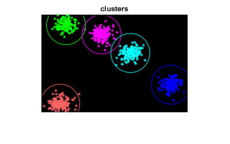
This program demonstrates kmeans clustering. It generates an image with random points, then assigns a random number of cluster centers and uses kmeans to move those cluster centers to their representitive location.
Sources:
Contents
Theory
We will explain with an example which is commonly used, the T-shirt size problem.
Consider a company, which is going to release a new model of T-shirt to market. Obviously they will have to manufacture models in different sizes to satisfy people of all sizes. So the company make a data of people's height and weight, and plot them on to a graph, as below:

Company can't create t-shirts with all the sizes. Instead, they divide people to Small, Medium and Large, and manufacture only these 3 models which will fit into all the people. This grouping of people into three groups can be done by k-means clustering, and algorithm provides us best 3 sizes, which will satisfy all the people. And if it doesn't, company can divide people to more groups, may be five, and so on. Check image below :

This algorithm is an iterative process. We will explain it step-by-step with the help of images.
Consider a set of data as below (you can consider it as t-shirt problem). We need to cluster this data into two groups.

Step 1: Algorithm randomly chooses two centroids, ![]() and
and ![]() (sometimes, any two data are taken as the centroids).
(sometimes, any two data are taken as the centroids).
Step 2: It calculates the distance from each point to both centroids. If a test data is more closer to ![]() , then that data is labelled with 0. If it is closer to
, then that data is labelled with 0. If it is closer to ![]() , then labelled as 1 (If more centroids are there, labelled as 2,|3| etc).
, then labelled as 1 (If more centroids are there, labelled as 2,|3| etc).
In our case, we will color all 0 labelled with red, and 1 labelled with blue. So we get following image after above operations.

Step 3: Next we calculate the average of all blue points and red points separately and that will be our new centroids. That is ![]() and
and ![]() shift to newly calculated centroids. (Remember, the images shown are not true values and not to true scale, it is just for
demonstration only).
shift to newly calculated centroids. (Remember, the images shown are not true values and not to true scale, it is just for
demonstration only).
And again, perform step 2 with new centroids and label data to 0 and 1. So we get result as below :

Now step 2 and 3 are iterated until both centroids are converged to fixed points. (Or it may be stopped depending on the criteria
we provide, like maximum number of iterations, or a specific accuracy is reached etc.). These points are such that sum of
distances between test data and their corresponding centroids are minimum. Or simply, sum of distances between ![]() and
and ![]() is minimum.
is minimum.
![]()
Final result almost looks like below :

So this is just an intuitive understanding of K-Means Clustering. For more details and mathematical explanation, please read any standard machine learning textbooks or check the links below. It is just a top layer of K-Means clustering. There are a lot of modifications to this algorithm like, how to choose the initial centroids, how to speed up the iteration process, etc.
- Machine Learning Course, Video lectures by Prof. Andrew Ng (some of the images are taken from it)
Initialization
% parameters
MAX_CLUSTERS = 5;
colorTab = [...
    0,   0, 255 ;
    0, 255,   0 ;
  255, 100, 100 ;
  255,   0, 255 ;
    0, 255, 255
];

% image on which to draw points
sz = [200 300];  % height/width, rows/cols
img = zeros([sz, 3], 'uint8');

% seed RNG for reproducible results
try, rng('default'); end
Data
choose number of samples and clusters
sampleCount = randi([1 1000]);
clusterCount = min(randi([2 MAX_CLUSTERS]), sampleCount);
generate random samples from multigaussian distribution
points = zeros([sampleCount,2], 'single');
idx = fix(linspace(1, sampleCount+1, clusterCount+1));
for i=1:numel(idx)-1
    center = [randi([0, sz(2)]) randi([0, sz(1)])];
    sigma = diag([sz(2) sz(1)]).*0.4;
    points(idx(i):idx(i+1)-1,:) = mvnrnd(center, sigma, idx(i+1)-idx(i));
end
show true labels
if mexopencv.isOctave()
    %HACK: http://savannah.gnu.org/bugs/?45497
    L = repelems(1:(numel(idx)-1), [1:(numel(idx)-1); diff(idx)]);
    %HACK: GSCATTER not implemented in Octave
    scatter(points(:,1), points(:,2), [], L)
else
    L = repelem(1:(numel(idx)-1), diff(idx));
    gscatter(points(:,1), points(:,2), L)
end
axis square equal ij
axis([1 sz(2) 1 sz(1)])

Clustering
shuffle points
points = points(randperm(sampleCount),:);
cluster points
[labels,centers,compactness] = cv.kmeans(points, clusterCount, ...
    'Criteria',struct('type','Count+EPS', 'maxCount',10, 'epsilon',0.1), ...
    'Attempts',3, 'Initialization','PP');
display(centers)
centers =
  5×2 single matrix
  265.1030  143.7113
   50.0097   21.1157
   38.3347  182.2368
  123.8976   40.6695
  182.8743   78.8241
compactness measure of clusters
%compactness = cv.norm(points, centers(labels+1,:), 'NormType','L2Sqr');
fprintf('Compactness = %f\n', compactness);
Compactness = 161486.122233
show clusters
img(:) = 0;
for i=1:sampleCount
    clusterIdx = labels(i)+1;
    img = cv.circle(img, points(i,:), 2, ...
        'Color',colorTab(clusterIdx,:), ...
        'Thickness','Filled', 'LineType','AA');
end
for i=1:clusterCount
    img = cv.circle(img, centers(i,:), 40, 'Color',colorTab(i,:), ...
        'Thickness',1, 'LineType','AA');
end
figure, imshow(img), title('clusters')
