K-Nearest Neighbors (KNN)

In this demo, we will understand the concepts of k-Nearest Neighbour (kNN) algorithm, then demonstrate how to use kNN classifier for 2D point classification.

Sources:

Contents

Theory

kNN is one of the simplest of classification algorithms available for supervised learning. The idea is to search for closest match of the test data in feature space. We will look into it with below image.

In the image, there are two families, Blue Squares and Red Triangles. We call each family as Class. Their houses are shown in their town map which we call feature space.

You can consider a feature space as a space where all datas are projected. For example, consider a 2D coordinate space. Each data has two features, x and y coordinates. You can represent this data in your 2D coordinate space, right? Now imagine if there are three features, you need 3D space. Now consider N features, where you need N-dimensional space, right? This N-dimensional space is its feature space. In our image, you can consider it as a 2D case with two features.

Now a new member comes into the town and creates a new home, which is shown as green circle. He should be added to one of these Blue/Red families. We call that process, Classification. What we do? Since we are dealing with kNN, let us apply this algorithm.

One method is to check who is his nearest neighbour. From the image, it is clear it is the Red Triangle family. So he is also added into Red Triangle. This method is called simply Nearest Neighbour, because classification depends only on the nearest neighbour.

But there is a problem with that. Red Triangle may be the nearest. But what if there are lot of Blue Squares near to him? Then Blue Squares have more strength in that locality than Red Triangle. So just checking nearest one is not sufficient. Instead we check some k nearest families. Then whoever is majority in them, the new guy belongs to that family. In our image, let's take k=3, i.e 3 nearest families. He has two Red and one Blue (there are two Blues equidistant, but since k=3, we take only one of them), so again he should be added to Red family. But what if we take k=7? Then he has 5 Blue families and 2 Red families. Great! Now he should be added to Blue family. So it all changes with value of k. More funny thing is, what if k=4? He has 2 Red and 2 Blue neighbours. It is a tie! So better take k as an odd number. So this method is called k-Nearest Neighbour since classification depends on k nearest neighbours.

Again, in kNN, it is true we are considering k neighbours, but we are giving equal importance to all, right? Is it justice? For example, take the case of k=4. We told it is a tie. But see, the 2 Red families are more closer to him than the other 2 Blue families. So he is more eligible to be added to Red. So how do we mathematically explain that? We give some weights to each family depending on their distance to the new-comer. For those who are near to him get higher weights while those are far away get lower weights. Then we add total weights of each family separately. Whoever gets highest total weights, new-comer goes to that family. This is called modified kNN.

So what are some important things you see here?

For additional resources, refer to:

Data

Form the training samples, randomly generated from two normal distributions

N = 100;  % number of training samples
data = [randn(N/2,2)*50+200 ; randn(N/2,2)*50+300];
labels = int32([ones(N/2,1)*1; ones(N/2,1)*2]);

whos data labels
if mexopencv.require('stats')
    tabulate(labels)
end

  Name          Size            Bytes  Class     Attributes

  data        100x2              1600  double              
  labels      100x1               400  int32               

  Value    Count   Percent
      1       50     50.00%
      2       50     50.00%

Train

Learn kNN classifier

K = 10;  % Try comparing K=1 (overfitting) vs. K=10 (more generalized)
knn = cv.KNearest();
knn.DefaultK = K;
tic
knn.train(data, labels);
toc

Elapsed time is 0.004994 seconds.

Performance on training set

acc = nnz(knn.predict(data) == labels) ./ N;
str = sprintf('Accuracy = %g%%',acc*100);
disp(str)

Accuracy = 92%

Predict

Build a grid of samples (2D points covering the data domain)

w = 500; h = 500;
[X,Y] = meshgrid(1:w, 1:h);
samples = [X(:) Y(:)];

Predict the responses and get the labels of all K nearest neighbors

tic
[pred,L] = knn.findNearest(samples, K);
toc

Elapsed time is 0.150778 seconds.

whos samples pred L
if mexopencv.require('stats')
    tabulate(pred)
end

  Name              Size               Bytes  Class     Attributes

  L            250000x10            10000000  single              
  pred         250000x1              1000000  single              
  samples      250000x2              4000000  double              

  Value    Count   Percent
      1    131337     52.53%
      2    118663     47.47%

Compute number of neighbors representing the majority, this indicates the prediction confidence on a [0,1] range (Note: for binary classification, it will never be less than 0.5, because it simply predicts the other class in such a case)

conf = sum(bsxfun(@eq, L, pred), 2) ./ K;

Reshaped as images

pred = reshape(pred, [h w]);
conf = reshape(conf, [h w]);

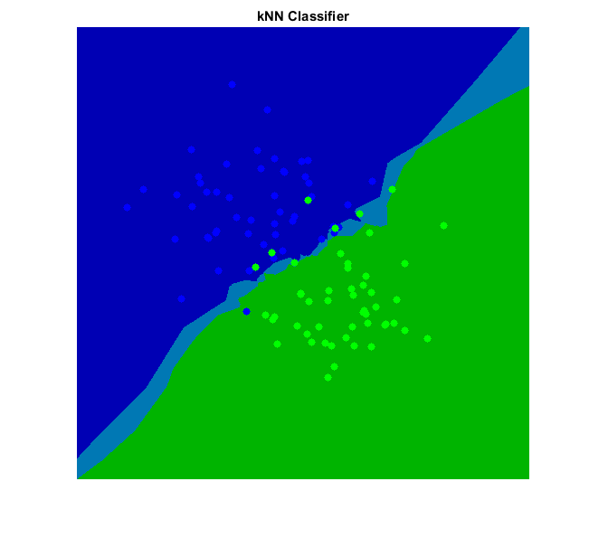
Plot 1

Highlight the pixels depending on the accuracy (or confidence)

cmap = [0 0 180; 0 180 0; 0 120 180; 0 120 120] ./ 255;
img = pred + (conf <= 0.5)*2;  % labels will be one of {1, 2, 3, 4}
img = ind2rgb(img, cmap);
img = uint8(img * 255);

Draw the original training samples

clr = [0 0 255; 0 255 0];
for i=1:2
    img = cv.circle(img, round(data(labels == i,:)), 4, ...
        'Color',clr(i,:), 'Thickness','Filled');
end

Show result

imshow(img), title('kNN Classifier')

Plot 2

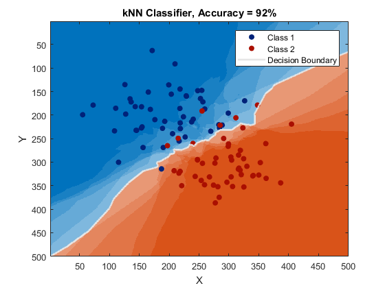
Show image color-coded by label, where transparency indicates confidence

clrBG = lines(2);
clrFG = brighten(clrBG, -0.6);
img = ind2rgb(pred, clrBG);
figure, hImg = image(img);
if ~mexopencv.isOctave()
    %HACK: transparency not yet implemented in Octave
    set(hImg, 'AlphaData',conf)
end
hold on
%scatter(data(:,1), data(:,2), [], clrFG(labels,:), 'filled')
for i=1:2
    scatter(data(labels==i,1), data(labels==i,2), [], clrFG(i,:), 'filled')
end
contour(pred, [1.5 1.5], 'LineWidth',2, 'LineColor',[1 1 1]*0.9)
hold off
xlabel('X'), ylabel('Y'), title(['kNN Classifier, ' str])
legend({'Class 1', 'Class 2', 'Decision Boundary'})