Image Segmentation with Distance Transform and Watershed Algorithm

Sample code showing how to segment overlapping objects using Laplacian filtering, in addition to Watershed and Distance Transformation.

In this demo you will learn how to:

Sources:

load image

fname = fullfile(mexopencv.root(), 'test', 'cards.png');
if exist(fname, 'file') ~= 2
    disp('Downloading image...')
    url = 'https://cdn.rawgit.com/opencv/opencv/3.2.0/samples/data/cards.png';
    urlwrite(url, fname);
end
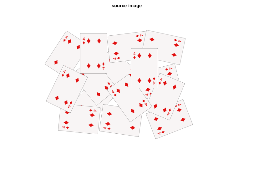
src = cv.imread(fname, 'Color',true);
imshow(src), title('source image')

change the background from white to black, since that will help later to extract better results during the use of Distance Transform

mask = all(src == 255, 3);
src(repmat(mask,[1 1 3])) = 0;
imshow(src), title('black background image')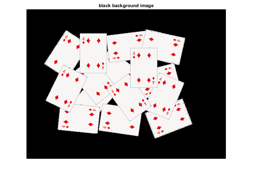

create a kernel that we will use for accuting/sharpening our image (an approximation of second derivative, a quite strong kernel)

if true
    kernel = [1 1 1; 1 -8 1; 1 1 1];
else
    kernel = [0 1 0; 1 -4 1; 0 1 0];
end

do the laplacian filtering, with intermediate calculations performed in floating-point precision (given the kernel used, Laplacian image will likely have negative values which would otherwise get truncated too soon)

if true
    imgLaplacian = cv.filter2D(src, kernel, 'DDepth','single');
else
    imgLaplacian = cv.Laplacian(src, 'DDepth','single');
end
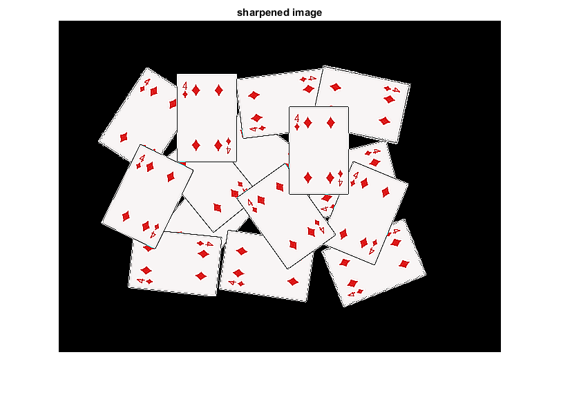
src = uint8(single(src) - imgLaplacian);
imshow(src), title('sharpened image')

create binary image from source image

bw = cv.cvtColor(src, 'RGB2GRAY');
bw = cv.threshold(bw, 'Otsu');
imshow(bw), title('binary')

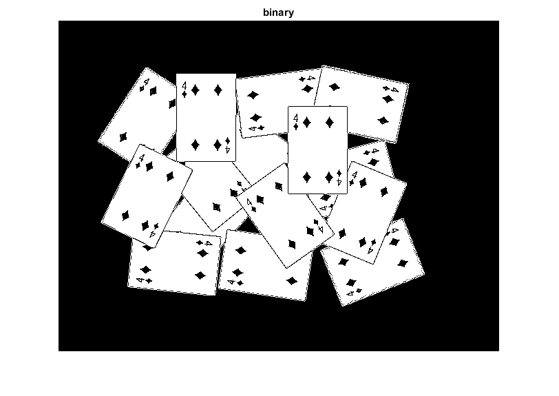
perform the distance transform algorithm, and normalize it to [0,1] range so we can visualize and threshold it

D = cv.distanceTransform(bw);
D = cv.normalize(D, 'Alpha',0, 'Beta',1, 'NormType','MinMax');
imshow(D), title('distance transform image')

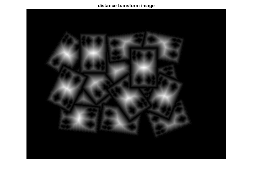
threshold distance image to obtain the peaks and dilate it a bit (these will be the markers for the foreground objects)

D = cv.threshold(D, 0.4, 'MaxValue',1);
D = cv.dilate(D);
imshow(D), title('peaks')
if ~mexopencv.isOctave()
    %HACK: transparency not yet implemented in Octave
    image('CData',src, 'AlphaData',0.3)
end

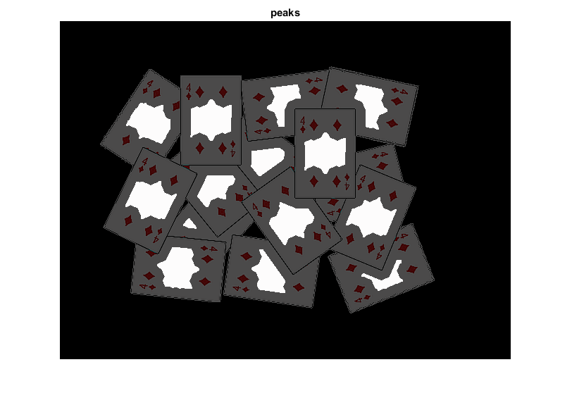
find total markers

D = uint8(D * 255);
contours = cv.findContours(D, 'Mode','External', 'Method','Simple');
contours = cellfun(@(C) cat(1,C{:}), contours, 'Uniform',false);
N = numel(contours);

create the marker image for the watershed algorithm and draw the markers (seed regions are marked with positive labels 1,2,3,etc. everything else 0)

markers = zeros(size(D), 'int32');

% foreground markers
for i=1:N
    markers = cv.drawContours(markers, contours, 'ContourIdx',i-1, ...
        'Color',i, 'Thickness','Filled');
end

% background marker
markers = cv.circle(markers, [5 5], 3, 'Color',N+1, 'Thickness','Filled');

perform the watershed algorithm

markers = cv.watershed(src, markers);

in output, pixels are assigned to regions (1,2,etc.), boundaries set to -1

L = uint8(markers);  % -1,1,2,..,N,N+1 -> 0,1,2,..,N,N+1
if ~mexopencv.isOctave() && mexopencv.require('stats')
    %HACK: tabulate in Octave behaves differently
    tabulate(L(:));  % 0=boundaries, 1:N=regions, N+1=background
end

  Value    Count   Percent
      0     5893      1.92%
      1     8805      2.87%
      2     9308      3.03%
      3     9914      3.23%
      4     2966      0.97%
      5    10354      3.37%
      6    13799      4.49%
      7    11038      3.59%
      8     6446      2.10%
      9     4272      1.39%
     10    10752      3.50%
     11     9412      3.06%
     12    10765      3.50%
     13     9432      3.07%
     14     8442      2.75%
     15    175602     57.16%

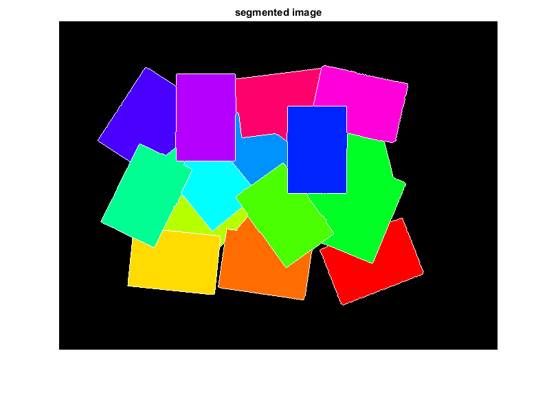
show segmented objects color-coded according to labels

clr = [1 1 1; hsv(N); 0 0 0];
rgb = uint8(255 * ind2rgb(L, clr));
imshow(rgb), title('segmented image')