cv.ANN_MLP - mexopencv

Artificial Neural Networks - Multi-Layer Perceptrons

Unlike many other models in ML that are constructed and trained at once, in the MLP model these steps are separated. First, a network with the specified topology is created. All the weights are set to zeros. Then, the network is trained using a set of input and output vectors. The training procedure can be repeated more than once, that is, the weights can be adjusted based on the new training data.

Neural Networks

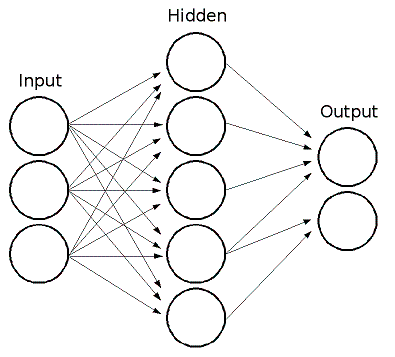
ML implements feed-forward artificial neural networks or, more particularly, multi-layer perceptrons (MLP), the most commonly used type of neural networks. MLP consists of the input layer, output layer, and one or more hidden layers. Each layer of MLP includes one or more neurons directionally linked with the neurons from the previous and the next layer. The example below represents a 3-layer perceptron with three inputs, two outputs, and the hidden layer including five neurons:

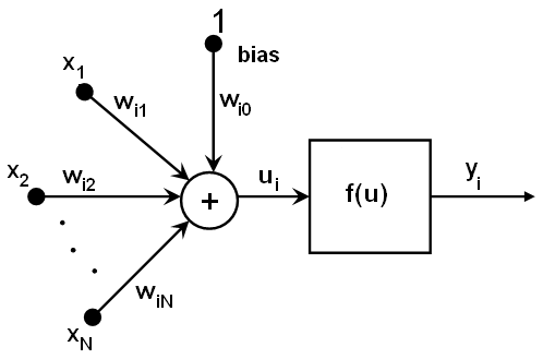
All the neurons in MLP are similar. Each of them has several input links (it takes the output values from several neurons in the previous layer as input) and several output links (it passes the response to several neurons in the next layer). The values retrieved from the previous layer are summed up with certain weights, individual for each neuron, plus the bias term. The sum is transformed using the activation function f that may be also different for different neurons.

In other words, given the outputs x_j of the layer n, the outputs y_i of the layer n+1 are computed as:

u_i = sum_j (w_{i,j}^{n+1} * x_j) + w_{i,bias}^{n+1}
y_i = f(u_i)

Different activation functions may be used. ML implements three standard functions:

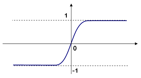
Identity: Identity function f(x) = y
Sigmoid: Symmetrical sigmoid, which is the default choice for MLP f(x) = beta * (1-exp(-alpha*x)) / (1+exp(-alpha*x))
Gaussian: Gaussian function, which is not completely supported at the moment f(x) = beta * exp(-alpha*x*x)

In ML, all the neurons have the same activation functions, with the same free parameters (alpha, beta) that are specified by user and are not altered by the training algorithms.

So, the whole trained network works as follows:

Take the feature vector as input. The vector size is equal to the size of the input layer.
Pass values as input to the first hidden layer.
Compute outputs of the hidden layer using the weights and the activation functions.
Pass outputs further downstream until you compute the output layer.

So, to compute the network, you need to know all the weights w_{i,j}^{n+1}. The weights are computed by the training algorithm. The algorithm takes a training set, multiple input vectors with the corresponding output vectors, and iteratively adjusts the weights to enable the network to give the desired response to the provided input vectors.

The larger the network size (the number of hidden layers and their sizes) is, the more the potential network flexibility is. The error on the training set could be made arbitrarily small. But at the same time the learned network also learn the noise present in the training set, so the error on the test set usually starts increasing after the network size reaches a limit. Besides, the larger networks are trained much longer than the smaller ones, so it is reasonable to pre-process the data, using cv.PCA or similar technique, and train a smaller network on only essential features.

Another MPL feature is an inability to handle categorical data as is. However, there is a workaround. If a certain feature in the input or output (in case of n-class classifier for n>2) layer is categorical and can take M>2 different values, it makes sense to represent it as a binary tuple of M elements, where the i-th element is 1 if and only if the feature is equal to the i-th value out of M possible. It increases the size of the input/output layer but speeds up the training algorithm convergence and at the same time enables fuzzy values of such variables, that is, a tuple of probabilities instead of a fixed value.

ML implements two algorithms for training MLP's.The first algorithm is a classical random sequential back-propagation algorithm. The second (default) one is a batch RPROP algorithm.

References

[BackPropWikipedia]:

Back-propagation algorithm

[LeCun98]:

LeCun, L. Bottou, G.B. Orr and K.-R. Muller, "Efficient backprop", in Neural Networks Tricks of the Trade, Springer Lecture Notes in Computer Sciences 1524, pp.5-50, 1998.

[RPROP93]:

M. Riedmiller and H. Braun, "A Direct Adaptive Method for Faster Backpropagation Learning: The RPROP Algorithm", Proc. ICNN, San Francisco (1993).

Superclasses	handle
Sealed	false
Construct on load	false

ActivationFunction	Activation function for all neurons.
AnnealCoolingRatio	ANNEAL: cooling ratio. It must be > 0 and less than 1. Default value
AnnealFinalT	ANNEAL: final temperature. It must be >= 0 and less than
AnnealInitialT	ANNEAL: initial temperature. It must be >= 0. Default value is 10.0.
AnnealItePerStep	ANNEAL: iteration per step. It must be > 0. Default value is 10.
BackpropMomentumScale	BPROP: Strength of the momentum term (the difference between weights
BackpropWeightScale	BPROP: Strength of the weight gradient term.
LayerSizes	Integer vector specifying the number of neurons in each layer
RpropDW0	RPROP: Initial value `delta_0` of update-values `delta_ij`.
RpropDWMax	RPROP: Update-values upper limit `delta_max`.
RpropDWMin	RPROP: Update-values lower limit `delta_min`.
RpropDWMinus	RPROP: Decrease factor `eta_minus`.
RpropDWPlus	RPROP: Increase factor `eta_plus`.
TermCriteria	Termination criteria of the training algorithm.
TrainMethod	Training method of the MLP.
id	Object ID

	addlistener	Add listener for event.
	calcError	Computes error on the training or test dataset
	clear	Clears the algorithm state
	delete	Destructor
	empty	Returns true if the algorithm is empty
	eq	== (EQ) Test handle equality.
	findobj	Find objects matching specified conditions.
	findprop	Find property of MATLAB handle object.
	ge	>= (GE) Greater than or equal relation for handles.
	getDefaultName	Returns the algorithm string identifier
	getVarCount	Returns the number of variables in training samples
	getWeights	Returns neurons weights of the particular layer
	gt	> (GT) Greater than relation for handles.
	isClassifier	Returns true if the model is a classifier
	isTrained	Returns true if the model is trained
Sealed	isvalid	Test handle validity.
	le	<= (LE) Less than or equal relation for handles.
	listener	Add listener for event without binding the listener to the source object.
	load	Loads algorithm from a file or a string
	lt	< (LT) Less than relation for handles.
	ne	~= (NE) Not equal relation for handles.
	notify	Notify listeners of event.
	predict	Predicts response(s) for the provided sample(s)
	save	Saves the algorithm parameters to a file or a string
	setActivationFunction	Initialize the activation function for each neuron
	setTrainMethod	Sets training method and common parameters
	train	Trains/updates the MLP